Session 2: Hypothesis Testing
Slides used for this session are available here with links to the Jupyter Notebooks: Arbuthnot’s Sign Test for section 1, for Section 2 and for Section 3 below.
1. A Historical Introduction to Hypothesis Testing: Arbuthnot’s Sign Test
John Arbuthnot’s 1710 analysis of baptism records in London is considered one of the earliest examples of hypothesis testing in statistics. By examining 82 years of birth records, Arbuthnot observed a consistent pattern: in every single year, more boys than girls were baptized. He sought to determine whether this pattern could have arisen by pure chance.
Arbuthnot’s Original Test (1710)
Observation:
In every year of the 82-year period studied, more boys than girls were baptized.
Null Hypothesis (H₀):
Each year, boys and girls are equally likely to be more numerous (p = 0.5).
Arbuthnot’s Argument:
- Under the null hypothesis, the probability that boys > girls in a single year is 0.5
- Since all n = 82 years showed more boys, the probability of this occurring by chance is:
This extraordinarily small probability (approximately 1 in 4.836 × 10²⁴) was computed by Arbuthnot as shown below:
 It led Arbuthnot to reject the null hypothesis and conclude that the excess of male births was not due to chance, but reflected a genuine phenomenon in nature.
The General Sign Test
Arbuthnot’s original case was unique because all years favored boys. However, the sign test can be generalized to situations where the pattern is not perfectly consistent.
Observation:
In each year, the number of boys and girls baptized is recorded. Some years have more boys, some years have more girls.
Null Hypothesis (H₀):
Each year, boys and girls are equally likely to be more numerous (probability = 0.5).
Procedure:
- Count the total number of years: n
- Count the number of years k where boys > girls
- Under H₀, the number X of “boy-favored” years follows a Binomial(n, 0.5) distribution
- Compute the probability of observing k or more boy-favored years using a one-sided binomial test:
Interpretation:
- If the p-value is small (typically < 0.05), we reject the null hypothesis and conclude that the observed excess of boys is statistically significant
- If the p-value is large, we fail to reject the null hypothesis – the observed pattern could reasonably occur by chance under H₀
- This generalizes Arbuthnot’s original argument to datasets where some years have more girls than boys (see Arbuthnot’s Sign Test for some numerical “simulations”)
Understanding Hypotheses in Statistical Science
What is a hypothesis?
A hypothesis in statistical science is not an absolute truth, but rather:
- A provisional, working assumption that guides our investigation
- A tentative explanation that can be tested against empirical evidence
- Within statistical science specifically: a particular assumption about a statistical model
- Example: In Arbuthnot’s test, the hypothesis that p = 0.5 (boys and girls are equally likely each year)
What is the null hypothesis?
The null hypothesis (H₀) is:
- The simplified statistical model that we work with until we have sufficient evidence against it
- A baseline or default position that represents “no effect” or “random chance”
- The hypothesis that we attempt to reject through statistical testing
- Example: In Arbuthnot’s test, H₀ states that “each year, boys and girls are equally likely to be more numerous”
The Logic of Hypothesis Testing
As Ronald Fisher eloquently stated in The Design of Experiments (1935):
“The null hypothesis is never proved or established, but is possibly disproved, in the course of experimentation. Every experiment may be said to exist only in order to give the facts a chance of disproving the null hypothesis.”
This fundamental principle highlights that:
- We cannot prove the null hypothesis is true—we can only fail to disprove it
- Statistical tests are designed to potentially reject the null hypothesis, not to confirm it
- The burden of proof lies in demonstrating that the data are inconsistent with the null hypothesis
- When we reject H₀, we conclude that the observed pattern is unlikely to have occurred by chance alone under H₀
2. Testing Independence in Contingency Tables: The Chi-Square Test
Introduction
This example examines the relationship between gender and arm-crossing preference (which arm goes on top when crossing arms). The data comes from a class survey of 54 students (source: Chapter 10 of The Art of Statistics by David Spiegelhalter):
- 14 females and 40 males
- 22 students cross their left arm on top
- 32 students cross their right arm on top
The “fundamental” question: Is arm-crossing preference independent of gender, or is there an association between these variables?
The Data: A 2×2 Contingency Table
| Left arm on top | Right arm on top | Total | |
|---|---|---|---|
| Female | 5 | 9 | 14 |
| Male | 17 | 23 | 40 |
| Total | 22 | 32 | 54 |
Observed proportions:
- Total population crossing right arm on top: 32/54 = 59%
- Females crossing right arm on top: 9/14 = 64.3%
- Males crossing right arm on top: 23/40 = 57.5%
- Difference in proportions: 64.3% - 57.5% = 6.8 percentage points
Null Hypothesis
H₀: Gender and arm-crossing preference are independent.
Under this hypothesis, the probability that someone crosses their right arm on top is the same regardless of gender. Is the observed difference of 6.8 % big enough to provide evidence against the null hypothesis?
Approach 1: Permutation Test (Randomization)
Concept
If gender and arm-crossing are truly independent, we could randomly shuffle who has which arm-crossing preference while keeping the gender composition fixed, and the resulting distribution would show us what differences we’d expect by chance.
Procedure
- Keep the gender labels fixed (14 females, 40 males)
- Keep the total counts fixed (22 left-arm crossers, 32 right-arm crossers)
- Randomly assign arm-crossing behaviors to individuals
- Calculate the proportion difference for each random assignment
- Repeat many times (e.g., 1,000 iterations) to build a null distribution
Interpretation
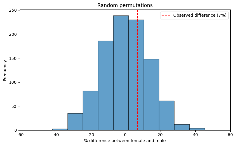
The resulting distribution shows all possible differences that could occur purely by chance under the null hypothesis. We compare our observed difference (6.8% $\approx$ 7%) to this distribution. If the observed difference is common in the randomization distribution, it’s consistent with chance. If it’s rare, we have evidence against independence.
Approach 2: Hypergeometric Distribution (Exact Permutations)
The “Balls in Urns” Analogy
Instead of randomly sampling permutations, we can calculate the exact probability of all possible outcomes:
- Imagine 54 balls: 14 white (females) and 40 black (males)
- Randomly draw 32 balls without replacement (representing the 32 people who cross right arm on top)
- Question: How many of the 32 drawn balls will be white?
Mathematical Framework
Under the null hypothesis of independence, the number of females crossing their right arm on top follows a hypergeometric distribution:
\[P(X = k) = \frac{\binom{14}{k}\binom{40}{32-k}}{\binom{54}{32}}\]where:
- X = number of females crossing right arm on top
- k ranges from 0 to 14
- The formula counts all ways to select k females and (32-k) males from the population
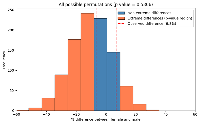
Two-sided Test
To test if the observed pattern (a difference of 6.8% in proportions) is unlikely under the null hypothesis, we need to define what “as extreme or more extreme” means in either direction.
| The most principled approach measures extremeness by the absolute difference in proportions. Here the observed difference is | 64.3% - 57.5% | = 6.8% |
The two-sided p-value is the sum of probabilities for all outcomes with absolute difference ≥ 6.8%:
\[P(\text{two-sided}) = \sum_{k: |d(k)| \geq |d_{\text{obs}}|} P(X = k)\]where:
- $d(k) = \frac{k}{14} - \frac{32-k}{40}$ is the difference in proportions when k females cross right arm on top
- $d_{\text{obs}} = \frac{9}{14} - \frac{23}{40}$ is the observed difference
- $P(X = k) = \frac{\binom{14}{k}\binom{40}{32-k}}{\binom{54}{32}}$ is the hypergeometric probability
Approach 3: Chi-Square Test
The Chi-Square Statistic
The chi-square test is the most commonly used method for testing independence in contingency tables. The test statistic quantifies how much the observed data differs from what we’d expect if there was no association.
Mathematical Formula
\[\chi^2 = \sum_{\text{all cells}} \frac{(\text{Observed} - \text{Expected})^2}{\text{Expected}}\]Calculation Steps
- Calculate expected frequencies under the null hypothesis of independence:
For our example:
- Expected females crossing right arm on top: (14 × 32) / 54 = 8.296
- Expected females crossing left arm on top: (14 × 22) / 54 = 5.704
- Expected males crossing right arm on top: (40 × 32) / 54 = 23.704
- Expected males crossing left arm on top: (40 × 22) / 54 = 16.296
- Calculate the chi-square statistic by summing contributions from all cells:
| Cell | Observed (O) | Expected (E) | (O - E)² / E |
|---|---|---|---|
| Female, Right | 9 | 8.296 | 0.0597 |
| Female, Left | 5 | 5.704 | 0.0868 |
| Male, Right | 23 | 23.704 | 0.0209 |
| Male, Left | 17 | 16.296 | 0.0304 |
Interpretation
- Small χ²: Observed data close to expected → little evidence against independence
- Large χ²: Observed data far from expected → strong evidence of association
- The chi-square statistic follows a χ² distribution with degrees of freedom = (rows - 1) × (columns - 1) = 1
For our data, χ² = 0.1978 is quite small, suggesting the observed difference is consistent with chance.
Important Consideration: Yates’ Continuity Correction
The Problem
The chi-square test approximates a discrete distribution (the actual data) with a continuous distribution (the χ² distribution). For small sample sizes or 2×2 tables, this can overestimate statistical significance.
The Solution: Yates’ Correction
Yates’ continuity correction adjusts the chi-square formula to be more conservative:
\[\chi^2_{\text{Yates}} = \sum_{\text{all cells}} \frac{(|O - E| - 0.5)^2}{E}\]The correction subtracts 0.5 from the absolute difference before squaring, reducing the chi-square statistic.
When to Use It
- Use correction: For 2×2 tables, especially with small expected frequencies (< 5 in any cell)
- Don’t use correction: For larger tables or when expected frequencies are all reasonably large
Important Note on Software Defaults
Be careful with default values in statistical software! Many implementations (including SciPy’s chi2_contingency) apply Yates’ correction by default for 2×2 tables. You may need to explicitly disable it (correction=False) to get the uncorrected test.