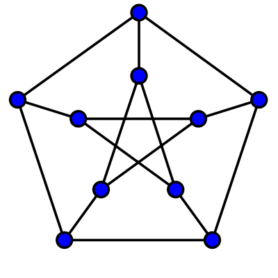
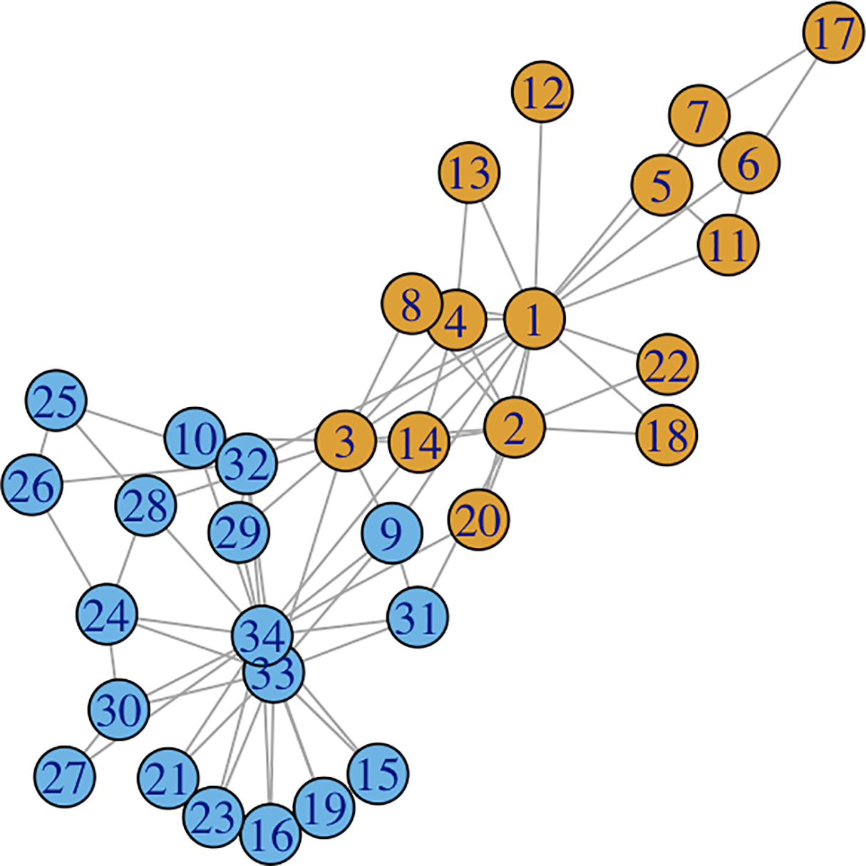
Graph Neural Networks [Marc Lelarge]

class: center, middle, title-slide
count: false

# A short introduction to Graph Neural Networks

<br/><br/>
.bold[Marc Lelarge]

---

# Motivation

- How to deal with structured data like graphs

- Examples of tasks:

- link prediction, node classification. Dataset = one large graph

- graph classification. Dataset = many small graphs (molecules, ego networks...)

--
count: false

- Idea: build a dense representation of the nodes/graph using message passing on edges.

--
count: false

- This is not new! Think for example of Pagerank...

--
count: false

- ... but here we will learn the message passing function!

---

# Warning: graphs are not images!

Result of seeing an image where nodes are pixels and where we
replace the grid by the complete graph:

.center.width-80[![](images/permuted_image.png)]

--
count: false

Extending the ideas of convolution is not completely straightforward.

---

# Graph Neural Networks

- start with initial node features $h_v^{(0)}$ for $v\in G$.

- after $k$ iterations, a node's representation captures the structural information within $k$-hop network neighborhood by:

$$
h_v^{(k)} = \phi\left(h_v^{(k-1)}, f \left( h_u^{(k-1)}, u\in\mathcal{N}(v) \right) \right),
$$
where:
 - $f$ is called the aggregate function and is **permutation invariant**
 - $\phi$ is the combine funtion.

---

# Representations used for prediction

- For node classification, the node representationh $h_v^{(K)}$ of the final iteration is used for prediction.

- For graph classification, we add a $\text{READOUT}$ function such that prediction is made tanks to

$$
h_G = \text{READOUT}\left( h_v^{(K)}, v\in G\right),
$$

where $\text{READOUT}$ is **permutation invariant**

--
count: false

### Property:

2 isomorphic graphs will have the same representation.

---

# Learning procedure

The functions $\phi$, $f$ and $\text{READOUT}$ are parametrized by neural networks (with the constraint of being permutation invariant for $f$ and $\text{READOUT}$).

For a given task, a loss is defined and the parameters of the functions $\phi$, $f$ and $\text{READOUT}$ are learned with a standard stochastic gradient procedure.

--
count: false

### Example: Graph Convolutional Networks

$$
h_v^{(k)} = \text{ReLU}\left( W \cdot \text{MEAN}\left( h_u^{(k-1)}, u\in\mathcal{N}(v)\cup {v}\right)\right)
$$

.citation[ [Thomas Kipf and Max Welling. Semi-supervised classification with graph convolutional networks. ICLR 2017](https://arxiv.org/abs/1609.02907)]

---

## Implementation with [DGL](https://docs.dgl.ai/en/latest/index.html)

.center.width-20[![](images/Petersen.png)]

You can create a DGL graph from networkx:

```
import networkx as nx
import dgl

g_nx = nx.petersen_graph()
g_dgl = dgl.DGLGraph(g_nx)

import torch

g.ndata['h'] = torch.randn(10,3) # assign one 3D vector to each node
```

---
## Convolutional layer

```
import torch.nn as nn

# Define the message & reduce function
def gcn_message(edges):
    # The argument is a batch of edges.
    # This computes a (batch of) message called 'msg' using the source node's feature 'h'.
    return {'msg' : edges.src['h']}

def gcn_reduce(nodes):
    # The argument is a batch of nodes.
    # This computes the new 'h' features by summing received 'msg' in each node's mailbox.
    return {'h' : torch.sum(nodes.mailbox['msg'], dim=1)}

# Define the GCNLayer module
class GCNLayer(nn.Module):
    def __init__(self, in_feats, out_feats):
        super(GCNLayer, self).__init__()
        self.linear = nn.Linear(in_feats, out_feats)

def forward(self, g, inputs):
        # g is the graph and the inputs is the input node features
        # first set the node features
        g.ndata['h'] = inputs
        # trigger message passing on all edges
        g.send(g.edges(), gcn_message)
        # trigger aggregation at all nodes
        g.recv(g.nodes(), gcn_reduce)
        # get the result node features
        h = g.ndata.pop('h')
        # perform linear transformation
        return self.linear(h)
```

---
## A 2-layer Graph Convolutional Network for node classification

```
# Define a 2-layer GCN model
class GCN(nn.Module):
    def __init__(self, in_feats, hidden_size, num_classes):
        super(GCN, self).__init__()
        self.gcn1 = GCNLayer(in_feats, hidden_size)
        self.gcn2 = GCNLayer(hidden_size, num_classes)

def forward(self, g, inputs):
        h = self.gcn1(g, inputs)
        h = torch.relu(h)
        h = self.gcn2(g, h)
        return h
# The first layer transforms input features of size of 34 to a hidden size of 5.
# The second layer transforms the hidden layer and produces output features of
# size 2, corresponding to the two groups.
net = GCN(34, 5, 2)
```

---
## Semi-supervised learning for the karate club

.center.width-70[![](images/KIDS-KARATE.jpg)]

---
## Semi-supervised learning for the karate club

.center.width-20[![](images/karate_net.jpg)]

```
inputs = torch.eye(34) # one-hot vectors to initialize the node features
labeled_nodes = torch.tensor([0, 33])  # only the instructor and the president nodes are labeled
labels = torch.tensor([0, 1])  # their labels are different

optimizer = torch.optim.Adam(net.parameters(), lr=0.01)
all_logits = []
for epoch in range(30):
    logits = net(G, inputs)
    logp = F.log_softmax(logits, 1)
    # we only compute loss for labeled nodes
    loss = F.nll_loss(logp[labeled_nodes], labels)
    optimizer.zero_grad()
    loss.backward()
    optimizer.step()
    print('Epoch %d | Loss: %.4f' % (epoch, loss.item()))
```

---

## Results

.center[
<img src="images/karate.gif" width="80%" />
]

.citation[source: Tutorial [DGL at a Glance](https://docs.dgl.ai/en/latest/tutorials/basics/1_first.html)]

---
class: end-slide, center
count: false

The end.