Deep Learning on Graphs [Marc Lelarge]

class: center, middle, title-slide
count: false

# Deep Learning on Graphs<br/>
# an Introduction

<br/><br/>
.bold[Marc Lelarge]

.bold[[www.dataflowr.com](https://mlelarge.github.io/dataflowr-web/)]

---

# Node embedding

## Language model

### one fixed graph, no signal. Ex: community detection

--
count: false

# Signal processing on graphs

## Fourier analysis on graphs

### one fixed graph, various signals. Ex: classification of signals

--
count: false

# Inductive representations on graphs

## Graph isomorphism problem: Weisfeiler-Lehman test

### various graphs. Ex: classification of graphs

---

# Node embedding

## Language model

### one fixed graph, no signal. Ex: community detection

- [DeepWalk](https://arxiv.org/abs/1403.6652)

- hierarchical softmax

- [node2vec](https://snap.stanford.edu/node2vec/)

- negative sampling

---

# Language model

- goal: to estimate the likelihood of a specific sequence of words appearing in a corpus.

- formally: to maximize $p(w\_{n} \| w\_{1}, ... , w\_{n-1})$ where $w\_i$ are in the vocabulary $V$.

## skip-gram model

- from the text, construct $D$ the multiset of all word and context pairs: $(w,c)$.

- goal: maximize $\prod\_{(w,c)\in D} p(c\| w ; \theta)$ in the parameter $\theta$.

- parametrization of the conditional probability thanks to a softmax:

$$
p(c\|w; \theta) = \frac{e^{u\_c \cdot u\_w}}{\sum\_{c'\in C}e^{u\_{c'} \cdot u\_w}},
$$
where $u\_c$ and $u\_w$ are vector representations for $c$ and $w$ and $C$ is the set of all available contexts.

---
# Hierarchical softmax

- Assign the contexts to the leaves of a binary tree and use the parametrization:

$$
p(c\|w; \theta) = \prod\_{b\in \pi(c)} \sigma(h\_b \cdot u\_w),
$$
where $\pi(c)$ is the path from the root to the leaf $c$ and $\sigma$ is the sigmoid function:

$$
\sigma(x) = \frac{1}{1+e^{-x}}.
$$

- reduce computational complexity from $O(|C|)$ to $O(\log|C|)$.

- speed up: assign shorter paths to frequent contexts using Huffman coding.

---

# DeepWalk

- a sentence = a random walk on the graph

--
count: false

---

# Negative sampling

- introduce $B = \mathbf{1}((w,c)\in D)$ with the parameterization

$$
p(b=1|w,c,\theta) = \sigma(u\_w \cdot u\_c)=\frac{1}{1+e^{-u\_w \cdot u\_c}} .
$$

- instead of maximizing $\prod\_{(w,c)\in D} p(c\| w ; \theta)$, we now maximize $\prod\_{(w,c)\in D} p(b=1 |c, w ; \theta)$

--
count: false

Problem, this has a trivial solution! We only have positive examples!

--
count: false

- create negative examples $D'$ and maximize in $\theta$:

$$
\sum\_{(w,c)\in D}\log \sigma(u\_w \cdot u\_c) + \sum_{(w,c)\in D'}\log \sigma(-u\_w \cdot u\_c)
$$

- in [Mikolov et al.](http://papers.nips.cc/paper/5021-distributed-representations-of-words-andphrases) $D'$ is $k$ times larger than $D$, and for each $(w,c)\in D$, we construct $k$ samples $(w,c\_1) ... (w,c\_k)$ where $c\_i$ is drawn according to its empirical distribution raised to the $3/4$ power.

---

# node2vec

- parameterization of the skip-gram model approximated thanks to negative sampling

- notion of context obtained thanks to biased random walk.

.center.width-50[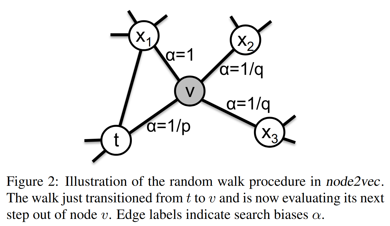![](images/node2vec_rw.png)]

---

# some results

.center.width-40[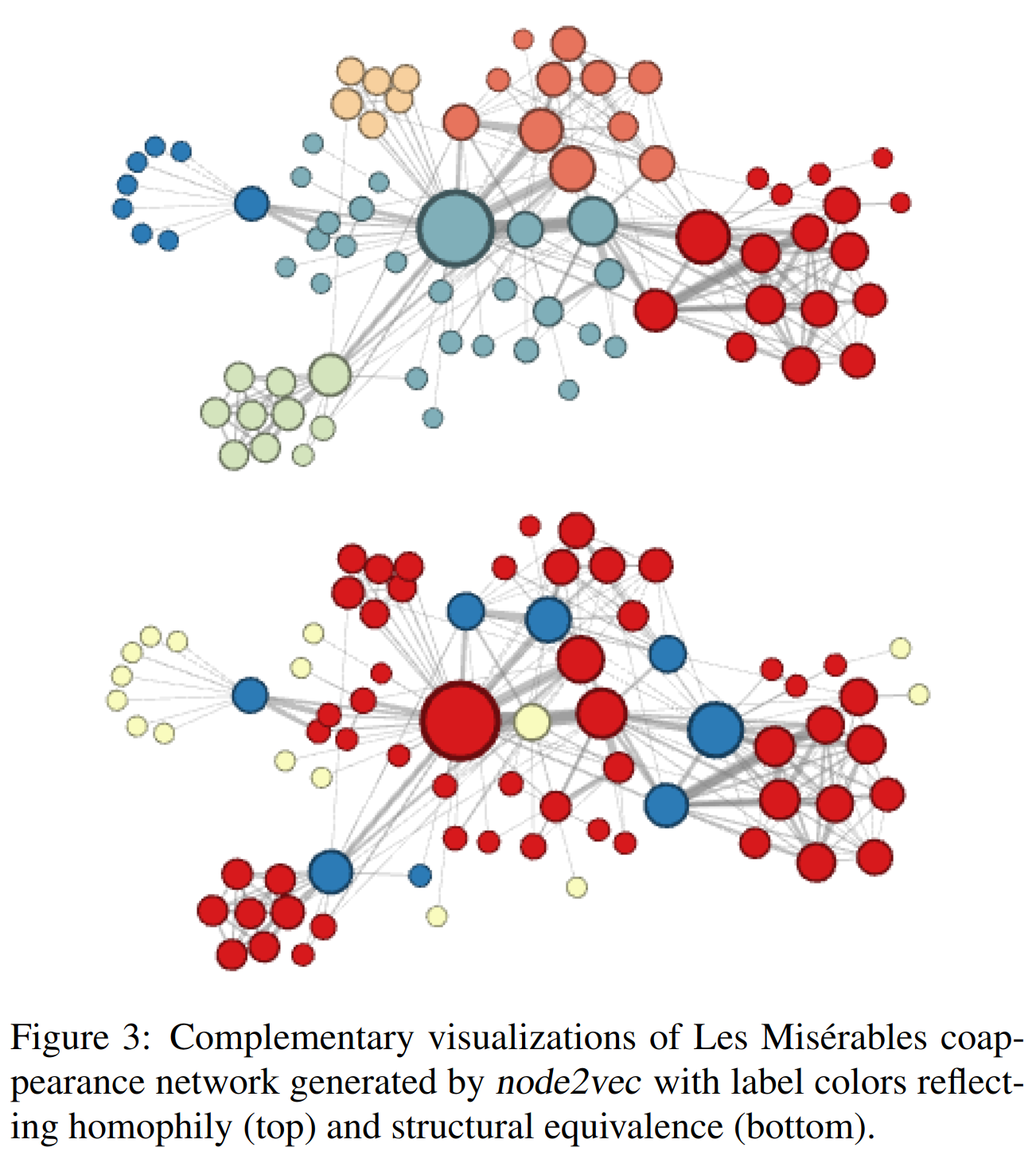![](images/node2vec_miserables.png)]

---
# some results

In the multi-label classification setting, every node is assigned one or more labels from a finite set. During training phase, a certain fraction of nodes with all their labels is observed. The task is to predict the labels for the remaining nodes.

.center.width-50[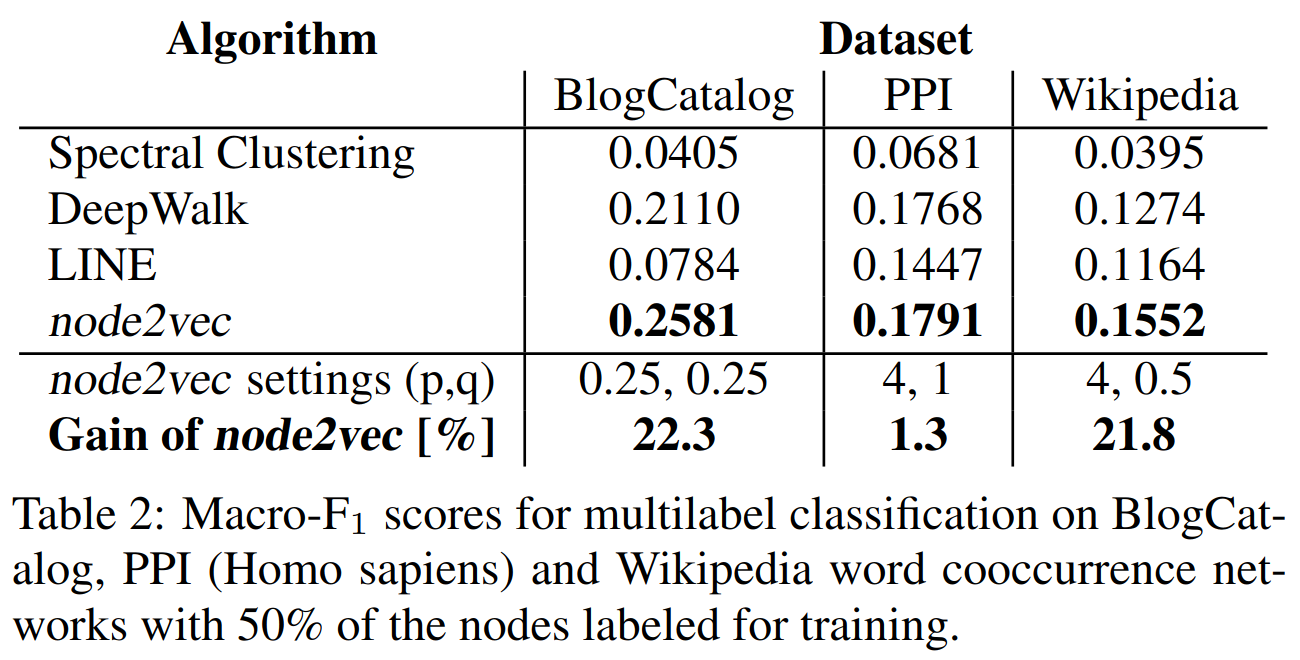![](images/node2vec_res.png)]

---
# Signal processing on graphs

## Fourier analysis on graphs

### one fixed graph, various signals. Ex: classification of signals

## Problem: how to implement a band-pass filter on a grah?

We first need to define a notion of frequency domain for graphs.

This will allow us to define convolutions on graphs.

---
# Recap: Fourier analysis

For (smooth) $f:\mathbb{R}^d \to \mathbb{C}$, we define the Fourier transform:
$$
\hat{f} (\xi) = \int f(x) e^{-2i\pi x\cdot \xi} dx,
$$
so that we have $f(x) = \int \hat{f}(\xi) e^{2i\pi x\cdot \xi} d\xi$.

The Fourier transform is a systematic way to decompose ''generic'' functions into a superposition of ''symmetric'' functions.
Here, the ''symmetric'' fucntions are plane waves with frequency $\xi$ defined by $e^{2i\pi x\cdot \xi}$ and can be seen as the eigenfunctions of the Laplacian on $\mathbb{R}^d$:
$$
f\mapsto \Delta f = \sum\_{i=1}^d\frac{\partial^2 f}{\partial x\_i^2}.
$$
Indeed $\Delta e^{2i\pi x\cdot \xi} = -4\pi^2|\xi|^2 e^{2i\pi x\cdot \xi}$.

The Fourier transform allows us to write an arbitrary function as a superposition of eigenfunctions of the Laplacian. This apporach works for general graphs!

---
# Spectral graph theory

For a graph $G=(V,E)$, we denote by $A$ its adjacency matrix and we define its Laplacian by $L=D-A$ where $D = \text{diag}(A 1)$ is the diagonal matrix of (weighted) degrees.

## Basics of $L$

We have $v^{T} L v = \sum\_{i < j} A\_{i,j}(v\_i -v\_j)^2$, $L 1=0$ and:
let $\lambda\_1=0\leq \lambda\_2\leq ... \leq \lambda\_n$ be the eigenvalues of the Laplacian, then $\lambda\_2>0$ if and only if $G$ is connected.

--
count: false

## Fiedler's nodal domain Theorem

Let $\lambda\_1=0< \lambda\_2\leq ... \leq \lambda\_n$ be the eigenvalues of the Laplacian of a connected graph $G$ and let $(u\_1,..., u\_n)$ be the corresponding eigenvectors.
For any $k\geq 2$, let
$$
W\_k = \\{ i \in V: u_k(i) \geq 0 \\}.
$$
Then, the graph induced by $G$ on $W\_k$ has at most $k-1$ connected components.
		     
---
# Graph Fourier transform  
				 
For a connected graph $G$ with $n$ vertices, we write the spectral decomposition of $L = U\Lambda U^T$, where
$$
\Lambda = \text{diag}(\lambda_1=0,\lambda_2,..., \lambda_n), \text{ and } U = (u\_1, ..., u\_n),
$$
with $U^TU = U U^T = Id$.

For a signal $f\in \mathbb{R}^n$, we define by $\hat{f}(\ell) = u\_{\ell}^T f$ its Fourier mode associated with frequency $\lambda\_{\ell}$. The Fourier transform of $f$ is given by
$$
\hat{f} = U^T f,
$$
so that we get
$$
f = U\hat{f} = \sum\_{\ell} \hat{f}(\ell) u\_{\ell}.
$$

---
# Filtering
##convolution = product in spectral domain

.center.width-60[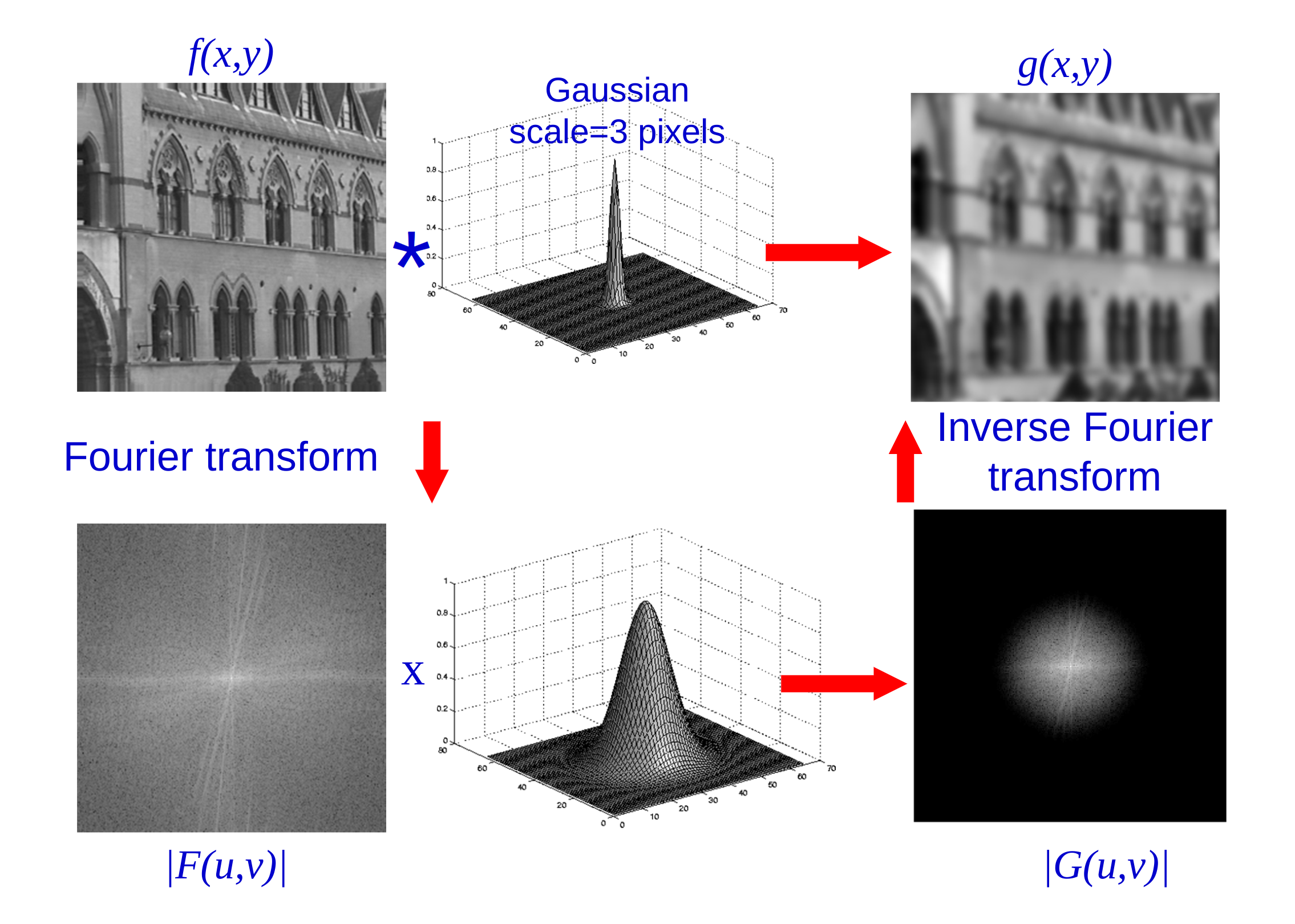![](images/fourier_ox.png)]

.citation[slide by Andrew Zisserman]

---
# Filtering on graphs

For a kernel function $k:\mathbb{R}^+ \to \mathbb{R}^+$ acting on the frequency domain, we define the operator $T\_k$ acting on a given signal $f$ as:
$$
\widehat{T\_k f}(\ell) = k(\lambda\_{\ell} )\hat{f}(\ell).
$$
In matrix form, we write (with $\odot$ the componentwise product):
$$
\widehat{T\_k f} = k(\Lambda) \odot \hat{f}.
$$

--
count: false

Going back in the spatial domain, we get:
$$\begin{aligned}
T\_k f & = U (k(\Lambda) \odot (U^T f))\\\\
&= U \text{diag}(k(\Lambda)) U^T f \\\\
& = k(L) f.
\end{aligned}$$

---

# Learning a localized kernel

In order to be able to learn our kernel, we will parametrize them and use polynomial kernels:
$$
k\_{\theta}(L) = \sum\_{k=0}^K \theta\_k L^k,
$$
where the parameter $\theta\in \mathbb{R}^K$ will be learned.

--
count: false

Note that if $d\_G(i,j)>K$, then we have $(L^K)\_{i,j} =0$, hence our kernel is $K$-localized.

Moreover, to compute the output of our filter, we need to evaluate:
$$
T\_k f = \sum\_{k=0}^K \theta\_k L^k f.
$$
This requires $K$ multiplication by a (sparse) matrix $L$ with a cost $O(K\|E\|)<< n^2$.

We defined a convolutional layer for graphs!

---

# Polynomial approximation

We are dealing with polynomial kernels. [Wavelets on graphs via spectral graph theory](https://arxiv.org/abs/0912.3848) suggests to use Chebyshev polynomial approximation.

The Chebyshev polynomials $T\_k(x)$ are generated by the recurrence:
$$
T\_k(x) = 2xT\_{k-1}(x) - T\_{k-2}(x),
$$
with $T\_0=1$ and $T\_1=x$. They are an orthogonal basis for $L^2([-1,1],dx/\sqrt{1-x^2})$ so that
$$
k(x) = c\_0/2 +\sum\_{k=1}^\infty c\_k T\_k(x),
$$
with Chebyshev coefficients
$$
c\_k = \frac{2}{\pi} \int\_{-1}^1 \frac{T\_k(x)k(x)}{\sqrt{1-x^2}}dx.
$$

---

# Polynomial approximation

.center.width-60[![](images/low-pass.png)]

Note: we shift the domain $[-1,1]$ to $[0,\lambda\_{\max}]$ using the transformation $y = \frac{\lambda\_{\max}(x+1)}{2}$. With the shifted Chebyshev polynomials $\overline{T}\_k(y) = T\_k(\frac{2y-\lambda\_{\max}}{\lambda\_{\max}})$, we parametrize the kernel by:
$$
k\_\theta(y) = \theta\_0 +\sum\_{k=1}^\infty \theta\_k \overline{T}\_k(y).
$$

.citation[source [Fast Eigenspace Approximation using Random Signals](https://arxiv.org/abs/1611.00938)]

---

# Convolutional neural networks on graphs

The paper [CNN on graphs with fast localized spectral filtering](https://arxiv.org/abs/1606.09375) introduces an additional pooling layer:

.center.width-60[![](images/pooling.png)]

--
count: false

### Performances on MNIST

Underlying graph: 8-NN graph of the 2D grid of size $28\times 28$ with weight
$W\_{i,j} = e^{-\||z\_i-z\_j\||^2/\sigma^2}$,
where $z\_i$ is the 2D coordinate of pixel $i$.

.center.width-60[![](images/mnist.png)]
---

# Semi-supervised learning for the karate club

.center.width-70[![](images/KIDS-KARATE.jpg)]

---
# Graph Convolutional Neural Networks
.center[
<img src="images/karate_4.png" width="50%" />
]

A two-layer GCN forward model is (with $\tilde{L}$ a renormalized version of the Laplacian):
$$
Z = f(X,A) = \text{softmax}(\tilde{L}\text{ ReLU}(\tilde{L}XW^{0})W^{1}),
$$
with $\tilde{L}\_{i,j} = 1/\sqrt{(d\_i+1)(d\_j+1)}$ for $i\sim j$ or $i=j$, and zero otherwise.

.citation[source [Semi-Supervised Classification with Graph Convolutional Networks](https://arxiv.org/abs/1609.02907)]

---

# Graph Convolutional Neural Networks
.center[
<img src="images/video.gif" width="50%" />
]

.citation[source [Semi-Supervised Classification with Graph Convolutional Networks](https://arxiv.org/abs/1609.02907)]

---

# Inductive representations on graphs

## Graph isomorphism problem: Weisfeiler-Lehman test

### various graphs. Ex: classification of graphs

--
count: false

Result of seeing an image where nodes are pixels and where we
replace the grid by the complete graph:

.center.width-80[![](images/permuted_image.png)]

---

# Invariant and equivariant linear operators

For an order-$k$ tensor $T\in \mathbb{R}^{n^k}$, we define for $\sigma\in \mathcal{S}\_n$:
$$
(\sigma \star T)\_{\sigma(i\_1),...,\sigma(i\_k)} = T\_{i\_1,...,i\_k}.
$$

A graph $G$ can be seen as a $2$-tensor. Two graphs $G\_1, G\_2$ are said isomorphic if there is a permutation $\sigma$ such that $G\_1=\sigma\star G\_2$.

--
count: false

A function $f:\mathbb{R}^{n^k}\to\mathbb{R}$ is said to be invariant if $f(\sigma \star T) = f(T)$ for every permutation $\sigma$.

A function $f:\mathbb{R}^{n^k}\to\mathbb{R^{n^\ell}}$ is said to be equivariant if $f(\sigma \star T) = \sigma\star f(T)$.

--
count: false

There is a basis of $b(k+\ell)$ possible equivariant linear operators $f:\mathbb{R}^{n^k}\to\mathbb{R^{n^\ell}}$.

The dimension of this space does not depend on the number of nodes $n$.

This allows applying the same network on graphs of different sizes!

.citation[[Invariant and Equivariant Graph Networks](https://arxiv.org/abs/1812.09902)]

---

# Invariant graph neural networks

A linear invariant function $f:\mathbb{R}^{n}\to\mathbb{R}$ is of the form $f(x) = \alpha 1^Tx$.

A linear equivariant function $f:\mathbb{R}^{n}\to\mathbb{R^n}$ is of the form $f(x) = [\alpha Id + \beta 11^T]x$.

A linear invariant function $f:\mathbb{R}^{n\times n}\to\mathbb{R}$ is of the form

--
count: false
$$
f(A) = \alpha\sum\_{ i =\not j } A\_{i,j} + \beta \sum\_{i=j}A\_{i,j}.
$$

In order to get more expressive layer, we need to use tensor of higher order.

[On the universality of invariant networks](https://arxiv.org/abs/1901.09342) shows that the minimal required order is $k\geq n^2$ in order to be able to approximate any invariant function.

This is of little practical value... we need another approach!

---
# The Weisfeiler-Lehman graph isomorphism test

.center.width-70[![](images/WL.png)]

---

# Graph Neural Networks

- start with initial node features $h_v^{(0)}$ for $v\in G$.

- after $k$ iterations, a node's representation captures the structural information within $k$-hop network neighborhood by:

$$
h_v^{(k)} = \phi\left(h_v^{(k-1)}, f \left( h_u^{(k-1)}, u\in\mathcal{N}(v) \right) \right),
$$
where:
 - $f$ is called the (local) aggregate function and is **permutation invariant**
 - $\phi$ is the combine funtion.

---

# Representations used for prediction

- For node classification, the node representationh $h_v^{(K)}$ of the final iteration is used for prediction.

- For graph classification, we add a $\text{READOUT}$ function such that prediction is made thanks to

$$
h_G = \text{READOUT}\left( h_v^{(K)}, v\in G\right),
$$

where $\text{READOUT}$ is **permutation invariant**

--
count: false

### Property:

2 isomorphic graphs will have the same representation.

---

# Learning procedure

The functions $\phi$, $f$ and $\text{READOUT}$ are parametrized by neural networks (with the constraint of being permutation invariant for $f$ and $\text{READOUT}$).

For a given task, a loss is defined and the parameters of the functions $\phi$, $f$ and $\text{READOUT}$ are learned with a standard stochastic gradient procedure.

--
count: false

### Example: Graph Convolutional Networks (seen previously)

$$
h_v^{(k)} = \text{ReLU}\left( W \cdot \text{MEAN}\left( h_u^{(k-1)}, u\in\mathcal{N}(v)\cup {v}\right)\right)
$$

--
count: false

### Example: Graph Isomorphism Network (GIN)

$$
h\_v^{(k)} = \text{MLP}^{(k)}\left( (1+\epsilon^{(k)}) h\_v^{(k-1)} + \sum\_{u\in\mathcal{N}(v)} h_u^{(k-1)}\right)
$$

.citation[ [How Powerful are Graph Neural Networks?](https://arxiv.org/abs/1810.00826)]

---
# Results

.center.width-80[![](images/result_GIN.png)]

---

## Implementation with [DGL](https://docs.dgl.ai/en/latest/index.html)

.center.width-20[![](images/Petersen.png)]

You can create a DGL graph from networkx:

```
import networkx as nx
import dgl

g_nx = nx.petersen_graph()
g_dgl = dgl.DGLGraph(g_nx)

import torch

g.ndata['h'] = torch.randn(10,3) # assign one 3D vector to each node
```

---
## Convolutional layer

```
import torch.nn as nn

# Define the message & reduce function
def gcn_message(edges):
    # The argument is a batch of edges.
    # This computes a (batch of) message called 'msg' using the source node's feature 'h'.
    return {'msg' : edges.src['h']}

def gcn_reduce(nodes):
    # The argument is a batch of nodes.
    # This computes the new 'h' features by summing received 'msg' in each node's mailbox.
    return {'h' : torch.sum(nodes.mailbox['msg'], dim=1)}

# Define the GCNLayer module
class GCNLayer(nn.Module):
    def __init__(self, in_feats, out_feats):
        super(GCNLayer, self).__init__()
        self.linear = nn.Linear(in_feats, out_feats)

def forward(self, g, inputs):
        # g is the graph and the inputs is the input node features
        # first set the node features
        g.ndata['h'] = inputs
        # trigger message passing on all edges
        g.send(g.edges(), gcn_message)
        # trigger aggregation at all nodes
        g.recv(g.nodes(), gcn_reduce)
        # get the result node features
        h = g.ndata.pop('h')
        # perform linear transformation
        return self.linear(h)
```

---
## A 2-layer Graph Convolutional Network for node classification

```
# Define a 2-layer GCN model
class GCN(nn.Module):
    def __init__(self, in_feats, hidden_size, num_classes):
        super(GCN, self).__init__()
        self.gcn1 = GCNLayer(in_feats, hidden_size)
        self.gcn2 = GCNLayer(hidden_size, num_classes)

def forward(self, g, inputs):
        h = self.gcn1(g, inputs)
        h = torch.relu(h)
        h = self.gcn2(g, h)
        return h
# The first layer transforms input features of size of 34 to a hidden size of 5.
# The second layer transforms the hidden layer and produces output features of
# size 2, corresponding to the two groups.
net = GCN(34, 5, 2)
```

---

## Semi-supervised learning for the karate club

.center.width-20[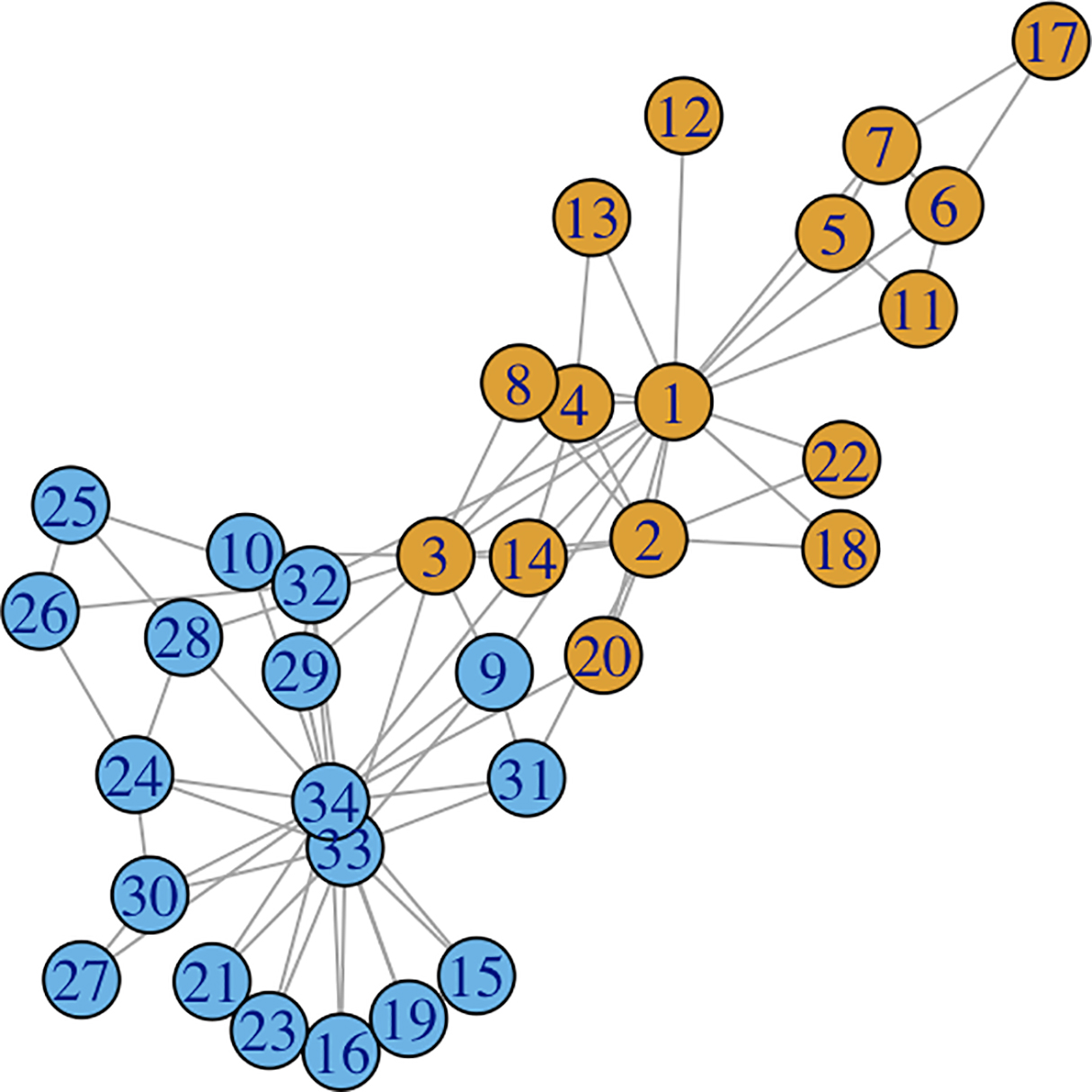![](images/karate_net.jpg)]

```
inputs = torch.eye(34) # one-hot vectors to initialize the node features
labeled_nodes = torch.tensor([0, 33])  # only the instructor and the president nodes are labeled
labels = torch.tensor([0, 1])  # their labels are different

optimizer = torch.optim.Adam(net.parameters(), lr=0.01)
all_logits = []
for epoch in range(30):
    logits = net(G, inputs)
    logp = F.log_softmax(logits, 1)
    # we only compute loss for labeled nodes
    loss = F.nll_loss(logp[labeled_nodes], labels)
    optimizer.zero_grad()
    loss.backward()
    optimizer.step()
    print('Epoch %d | Loss: %.4f' % (epoch, loss.item()))
```

---

## Results

.center[
<img src="images/karate.gif" width="80%" />
]

.citation[source: Tutorial [DGL at a Glance](https://docs.dgl.ai/en/latest/tutorials/basics/1_first.html)]
---

# Node embedding

## Language model

### one fixed graph, no signal. Ex: community detection

# Signal processing on graphs

## Fourier analysis on graphs

### one fixed graph, various signals. Ex: classification of signals

# Inductive representations on graphs

## Graph isomorphism problem: Weisfeiler-Lehman test

### various graphs. Ex: classification of graphs

---
class: end-slide, center
count: false

The end.